NumPy 高级功能与技巧

难度: 高级

numpy 高级功能网格生成数组操作性能优化

NumPy 高级功能与技巧

📝 概述

NumPy提供了许多高级功能和技巧，包括网格生成、高级索引、数组操作、性能优化等。本文档深入介绍这些高级特性，帮助您更高效地使用NumPy进行科学计算。

🎯 学习目标

掌握mgrid和meshgrid的使用方法
学会高级数组操作技巧
了解NumPy的性能优化方法
掌握数组的连接、分割和重塑
学会处理复杂的索引和选择操作

📋 前置知识

NumPy基础操作
数组索引和切片
基本的数学和几何概念
Python编程基础

🔍 详细内容

网格生成函数

mgrid函数详解

mgrid是NumPy中用于生成多维网格的强大工具，常用于创建坐标网格进行数值计算和可视化。

语法格式

np.mgrid[start:end:step]

参数说明：

start: 开始坐标
end: 结束坐标
step: 步长
- 实数步长：表示间隔，左闭右开区间
- 复数步长：表示点数，左闭右闭区间

一维网格生成

import numpy as np
import matplotlib.pyplot as plt

# 使用复数步长（指定点数）
x = np.mgrid[-5:5:5j]  # 生成5个点，从-5到5
print(f"5个点的网格: {x}")
# 输出: [-5.  -2.5  0.   2.5  5. ]

# 使用实数步长（指定间隔）
y = np.mgrid[0:10:2]  # 从0到10，步长为2
print(f"步长为2的网格: {y}")
# 输出: [0 2 4 6 8]

# 使用浮点步长
z = np.mgrid[0:1:0.2]
print(f"浮点步长网格: {z}")
# 输出: [0.  0.2 0.4 0.6 0.8]

二维网格生成

# 生成2D网格
x, y = np.mgrid[-2:3:3j, -1:2:3j]
print(f"X坐标网格:\n{x}")
print(f"Y坐标网格:\n{y}")

# X网格：每列相同（水平方向扩展）
# [[-2. -2. -2.]
#  [ 0.  0.  0.]
#  [ 2.  2.  2.]]

# Y网格：每行相同（垂直方向扩展）
# [[-1.  0.  1.]
#  [-1.  0.  1.]
#  [-1.  0.  1.]]

# 实际应用：计算每个网格点的函数值
z = x**2 + y**2  # 计算距离平方
print(f"距离平方网格:\n{z}")

三维网格生成

# 生成3D网格
x, y, z = np.mgrid[-1:2:2j, -1:2:2j, -1:2:2j]
print(f"3D网格形状: X{x.shape}, Y{y.shape}, Z{z.shape}")
print(f"X网格:\n{x}")
print(f"Y网格:\n{y}")
print(f"Z网格:\n{z}")

# 计算3D函数值
values = np.sqrt(x**2 + y**2 + z**2)  # 计算到原点的距离
print(f"距离值:\n{values}")

meshgrid函数对比

# meshgrid与mgrid的对比
x_1d = np.linspace(-2, 2, 3)
y_1d = np.linspace(-1, 1, 3)

# 使用meshgrid
X_mesh, Y_mesh = np.meshgrid(x_1d, y_1d)
print(f"meshgrid结果:")
print(f"X:\n{X_mesh}")
print(f"Y:\n{Y_mesh}")

# 使用mgrid
X_mgrid, Y_mgrid = np.mgrid[-2:2:3j, -1:1:3j]
print(f"\nmgrid结果:")
print(f"X:\n{X_mgrid}")
print(f"Y:\n{Y_mgrid}")

# 主要区别：meshgrid的X和Y是转置关系
print(f"\n形状对比:")
print(f"meshgrid: X{X_mesh.shape}, Y{Y_mesh.shape}")
print(f"mgrid: X{X_mgrid.shape}, Y{Y_mgrid.shape}")

网格的实际应用

三维函数绘图示例

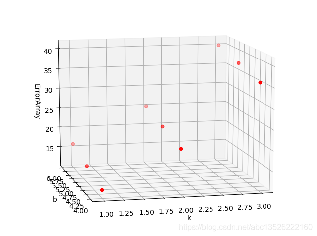
以下示例展示如何使用mgrid生成三维函数图像。考虑函数：

$数学公式$

其中k轴范围为1~3，b轴范围为4~6。

import numpy as np
import matplotlib.pyplot as plt
import mpl_toolkits.mplot3d.axes3d as p3

# 生成网格
k, b = np.mgrid[1:3:3j, 4:6:3j]
f_kb = 3*k**2 + 2*b + 1

# 绘制散点图
fig = plt.figure()
ax = p3.Axes3D(fig)
ax.scatter(k, b, f_kb, c='r')
ax.set_xlabel('k')
ax.set_ylabel('b')
ax.set_zlabel('ErrorArray')
plt.show()

三维散点图

# 绘制曲面图
ax = plt.subplot(111, projection='3d')
ax.plot_surface(k, b, f_kb, rstride=1, cstride=1)
ax.set_xlabel('k')
ax.set_ylabel('b')
ax.set_zlabel('ErrorArray')
plt.show()

三维曲面图

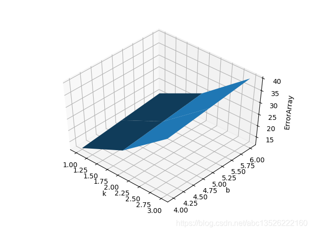
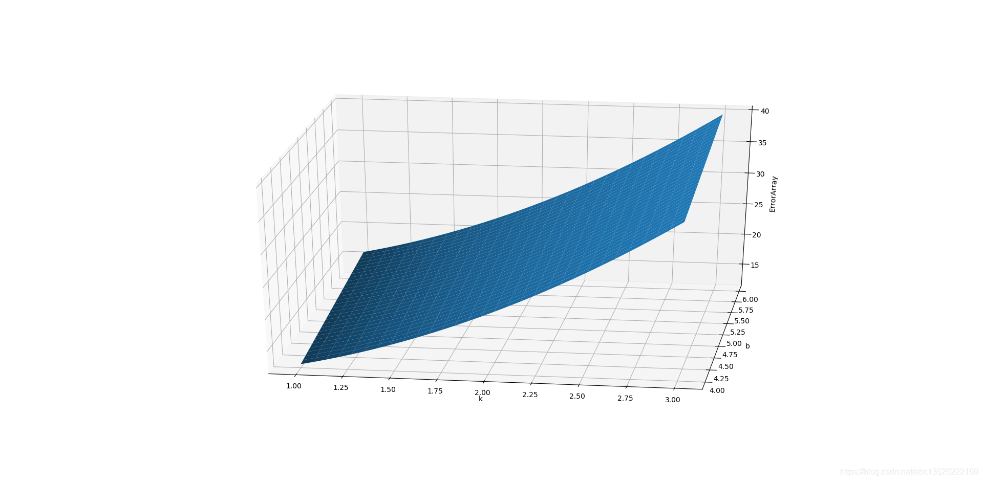
注意：mgrid中第三个参数（点数）越大，网格分割越细，曲面越精准。

使用10j参数的效果：
使用30j参数的效果：

# 应用1：绘制函数图像
def plot_function_2d():
    """绘制2D函数图像"""
    x, y = np.mgrid[-3:3:100j, -3:3:100j]
    
    # 定义函数
    z1 = np.sin(np.sqrt(x**2 + y**2))  # 波纹函数
    z2 = np.exp(-(x**2 + y**2)/2)      # 高斯函数
    z3 = x**2 - y**2                   # 鞍点函数
    
    return x, y, z1, z2, z3

# 应用2：数值积分网格
def numerical_integration_grid(func, x_range, y_range, n_points=50):
    """创建数值积分网格"""
    x, y = np.mgrid[x_range[0]:x_range[1]:n_points*1j, 
                    y_range[0]:y_range[1]:n_points*1j]
    
    # 计算函数值
    z = func(x, y)
    
    # 简单的数值积分（矩形法则）
    dx = (x_range[1] - x_range[0]) / (n_points - 1)
    dy = (y_range[1] - y_range[0]) / (n_points - 1)
    integral = np.sum(z) * dx * dy
    
    return integral

# 示例：计算高斯函数的积分
gaussian_2d = lambda x, y: np.exp(-(x**2 + y**2)/2)
integral_result = numerical_integration_grid(gaussian_2d, [-3, 3], [-3, 3])
print(f"高斯函数积分近似值: {integral_result:.4f}")
print(f"理论值: {2*np.pi:.4f}")

高级数组操作

数组连接和堆叠

# 创建示例数组
a = np.array([[1, 2], [3, 4]])
b = np.array([[5, 6], [7, 8]])
c = np.array([9, 10])

print(f"数组a:\n{a}")
print(f"数组b:\n{b}")
print(f"数组c: {c}")

# concatenate：沿指定轴连接
concat_0 = np.concatenate([a, b], axis=0)  # 垂直连接
concat_1 = np.concatenate([a, b], axis=1)  # 水平连接
print(f"\n垂直连接:\n{concat_0}")
print(f"水平连接:\n{concat_1}")

# vstack和hstack：垂直和水平堆叠
vstack_result = np.vstack([a, b])
hstack_result = np.hstack([a, b])
print(f"\nvstack结果:\n{vstack_result}")
print(f"hstack结果:\n{hstack_result}")

# column_stack：按列堆叠（自动转换1D为列向量）
column_result = np.column_stack([c, c*2])
print(f"\ncolumn_stack结果:\n{column_result}")

# dstack：按深度堆叠
dstack_result = np.dstack([a, b])
print(f"\ndstack结果形状: {dstack_result.shape}")
print(f"dstack结果:\n{dstack_result}")

数组分割

# 创建用于分割的数组
large_array = np.arange(24).reshape(4, 6)
print(f"原数组:\n{large_array}")

# split：沿指定轴分割
split_result = np.split(large_array, 2, axis=0)  # 分成2部分
print(f"\n按行分割:")
for i, part in enumerate(split_result):
    print(f"部分{i+1}:\n{part}")

# 指定分割位置
split_positions = np.split(large_array, [1, 3], axis=0)  # 在索引1和3处分割
print(f"\n指定位置分割:")
for i, part in enumerate(split_positions):
    print(f"部分{i+1}:\n{part}")

# hsplit和vsplit：水平和垂直分割
hsplit_result = np.hsplit(large_array, 3)  # 分成3列
vsplit_result = np.vsplit(large_array, 2)  # 分成2行

print(f"\n水平分割结果数量: {len(hsplit_result)}")
print(f"垂直分割结果数量: {len(vsplit_result)}")

数组重复和平铺

# repeat：重复元素
arr = np.array([1, 2, 3])
repeated = arr.repeat(3)  # 每个元素重复3次
print(f"repeat结果: {repeated}")

# 对多维数组按轴重复
arr_2d = np.array([[1, 2], [3, 4]])
repeated_axis0 = arr_2d.repeat(2, axis=0)  # 沿axis=0重复
repeated_axis1 = arr_2d.repeat(2, axis=1)  # 沿axis=1重复
print(f"\n原2D数组:\n{arr_2d}")
print(f"沿axis=0重复:\n{repeated_axis0}")
print(f"沿axis=1重复:\n{repeated_axis1}")

# tile：平铺数组
tiled = np.tile(arr, 3)  # 整个数组重复3次
print(f"\ntile结果: {tiled}")

# 多维平铺
tiled_2d = np.tile(arr_2d, (2, 3))  # 行重复2次，列重复3次
print(f"2D tile结果:\n{tiled_2d}")

高级索引技巧

花式索引的高级用法

# 创建示例数据
data = np.arange(20).reshape(4, 5)
print(f"原数据:\n{data}")

# 使用布尔数组和整数数组组合索引
row_mask = np.array([True, False, True, False])
col_indices = np.array([0, 2, 4])

# 选择特定行的特定列
selected = data[row_mask][:, col_indices]
print(f"\n选择结果:\n{selected}")

# 使用np.ix_进行网格索引
rows = np.array([0, 2])
cols = np.array([1, 3, 4])
grid_selected = data[np.ix_(rows, cols)]
print(f"\n网格索引结果:\n{grid_selected}")

# 条件索引
condition = (data > 5) & (data < 15)
conditional_selected = data[condition]
print(f"\n条件索引结果: {conditional_selected}")

where函数的高级应用

# where作为三元运算符
x = np.array([-2, -1, 0, 1, 2])
y = np.array([1, 2, 3, 4, 5])

# 条件选择
result = np.where(x > 0, x, y)  # x>0时选择x，否则选择y
print(f"条件选择结果: {result}")

# 多条件where
complex_result = np.where(x > 0, x**2, 
                         np.where(x < 0, -x, 0))
print(f"多条件结果: {complex_result}")

# where返回索引
indices = np.where(x > 0)
print(f"满足条件的索引: {indices[0]}")
print(f"满足条件的值: {x[indices]}")

# 二维数组的where
array_2d = np.array([[1, -2, 3], [-4, 5, -6]])
positive_indices = np.where(array_2d > 0)
print(f"\n2D数组正数位置:")
print(f"行索引: {positive_indices[0]}")
print(f"列索引: {positive_indices[1]}")
print(f"正数值: {array_2d[positive_indices]}")

唯一值和集合操作

# 创建示例数据
array1 = np.array([1, 2, 3, 2, 4, 1, 5])
array2 = np.array([2, 3, 4, 6, 7])

print(f"数组1: {array1}")
print(f"数组2: {array2}")

# unique：获取唯一值
unique_vals = np.unique(array1)
print(f"\n唯一值: {unique_vals}")

# 返回索引和计数
unique_vals, indices, counts = np.unique(array1, return_index=True, return_counts=True)
print(f"唯一值: {unique_vals}")
print(f"首次出现索引: {indices}")
print(f"出现次数: {counts}")

# 集合操作
intersection = np.intersect1d(array1, array2)  # 交集
union = np.union1d(array1, array2)            # 并集
difference = np.setdiff1d(array1, array2)     # 差集
sym_diff = np.setxor1d(array1, array2)        # 对称差集

print(f"\n交集: {intersection}")
print(f"并集: {union}")
print(f"差集(1-2): {difference}")
print(f"对称差集: {sym_diff}")

# 成员检查
membership = np.in1d(array1, array2)
print(f"\n成员检查: {membership}")
print(f"array1中在array2中的元素: {array1[membership]}")

排序和搜索

高级排序

# 创建示例数据
data = np.array([3, 1, 4, 1, 5, 9, 2, 6])
print(f"原数据: {data}")

# 基本排序
sorted_data = np.sort(data)
print(f"排序后: {sorted_data}")

# 获取排序索引
sort_indices = np.argsort(data)
print(f"排序索引: {sort_indices}")
print(f"验证: {data[sort_indices]}")

# 多维数组排序
data_2d = np.array([[3, 1, 4], [1, 5, 9], [2, 6, 5]])
print(f"\n2D数组:\n{data_2d}")

# 沿不同轴排序
sorted_axis0 = np.sort(data_2d, axis=0)  # 按列排序
sorted_axis1 = np.sort(data_2d, axis=1)  # 按行排序
print(f"按列排序:\n{sorted_axis0}")
print(f"按行排序:\n{sorted_axis1}")

部分排序和搜索

# partition：部分排序
data = np.array([3, 1, 4, 1, 5, 9, 2, 6, 5, 3])
print(f"原数据: {data}")

# 找到第k小的元素
k = 3
partitioned = np.partition(data, k)
print(f"第{k+1}小的元素: {partitioned[k]}")
print(f"部分排序结果: {partitioned}")

# argpartition：获取部分排序的索引
partition_indices = np.argpartition(data, k)
print(f"部分排序索引: {partition_indices}")

# 找到最小的k个元素
smallest_k = np.partition(data, k)[:k+1]
print(f"最小的{k+1}个元素: {np.sort(smallest_k)}")

# searchsorted：在已排序数组中搜索插入位置
sorted_array = np.array([1, 3, 5, 7, 9])
values_to_insert = [2, 4, 6, 8]
insert_positions = np.searchsorted(sorted_array, values_to_insert)
print(f"\n已排序数组: {sorted_array}")
print(f"要插入的值: {values_to_insert}")
print(f"插入位置: {insert_positions}")

性能优化技巧

向量化操作

import time

# 比较向量化和循环的性能
n = 1000000
a = np.random.randn(n)
b = np.random.randn(n)

# 方法1：Python循环（慢）
start_time = time.time()
result_loop = []
for i in range(n):
    result_loop.append(a[i] * b[i])
loop_time = time.time() - start_time

# 方法2：NumPy向量化（快）
start_time = time.time()
result_vectorized = a * b
vectorized_time = time.time() - start_time

print(f"循环方法耗时: {loop_time:.4f}秒")
print(f"向量化方法耗时: {vectorized_time:.4f}秒")
print(f"性能提升: {loop_time/vectorized_time:.1f}倍")

# 验证结果一致性
print(f"结果一致性: {np.allclose(result_loop, result_vectorized)}")

内存优化

# 就地操作减少内存使用
large_array = np.random.randn(1000, 1000)
print(f"原数组内存使用: {large_array.nbytes / 1024**2:.2f} MB")

# 避免创建临时数组
# 不好的做法：创建临时数组
# result = large_array + 1
# result = result * 2

# 好的做法：就地操作
large_array += 1  # 就地加法
large_array *= 2  # 就地乘法

# 使用out参数
result = np.empty_like(large_array)
np.add(large_array, 1, out=result)  # 指定输出数组

print(f"优化后内存使用更高效")

数据类型优化

# 选择合适的数据类型
data_int64 = np.arange(1000, dtype=np.int64)
data_int32 = np.arange(1000, dtype=np.int32)
data_int16 = np.arange(1000, dtype=np.int16)

print(f"int64内存使用: {data_int64.nbytes} bytes")
print(f"int32内存使用: {data_int32.nbytes} bytes")
print(f"int16内存使用: {data_int16.nbytes} bytes")

# 检查数据范围选择合适类型
data = np.array([1, 100, 255])
print(f"\n数据范围: {np.min(data)} - {np.max(data)}")
print(f"可以使用uint8: {np.max(data) <= 255}")

# 转换为更小的数据类型
data_optimized = data.astype(np.uint8)
print(f"优化前: {data.dtype}, 内存: {data.nbytes} bytes")
print(f"优化后: {data_optimized.dtype}, 内存: {data_optimized.nbytes} bytes")

💡 实际应用

图像处理应用

# 模拟图像处理
def create_synthetic_image(width=100, height=100):
    """创建合成图像"""
    x, y = np.mgrid[0:width, 0:height]
    
    # 创建渐变图像
    gradient = x / width + y / height
    
    # 创建圆形图案
    center_x, center_y = width // 2, height // 2
    circle = np.sqrt((x - center_x)**2 + (y - center_y)**2)
    circle_mask = circle < min(width, height) // 4
    
    # 组合图像
    image = gradient * 0.5 + circle_mask * 0.5
    
    return image

# 图像滤波
def apply_filter(image, filter_type='blur'):
    """应用简单滤波器"""
    if filter_type == 'blur':
        # 简单的3x3均值滤波
        kernel = np.ones((3, 3)) / 9
    elif filter_type == 'sharpen':
        # 锐化滤波器
        kernel = np.array([[-1, -1, -1],
                          [-1,  9, -1],
                          [-1, -1, -1]])
    
    # 应用卷积（简化版本）
    filtered = np.zeros_like(image)
    for i in range(1, image.shape[0]-1):
        for j in range(1, image.shape[1]-1):
            filtered[i, j] = np.sum(image[i-1:i+2, j-1:j+2] * kernel)
    
    return filtered

# 示例使用
image = create_synthetic_image()
blurred = apply_filter(image, 'blur')
sharpened = apply_filter(image, 'sharpen')

print(f"原图像统计: 均值={np.mean(image):.3f}, 标准差={np.std(image):.3f}")
print(f"模糊图像统计: 均值={np.mean(blurred):.3f}, 标准差={np.std(blurred):.3f}")
print(f"锐化图像统计: 均值={np.mean(sharpened):.3f}, 标准差={np.std(sharpened):.3f}")

科学计算应用

# 数值微分
def numerical_gradient(func, x, h=1e-5):
    """计算数值梯度"""
    grad = np.zeros_like(x)
    for i in range(len(x)):
        x_plus = x.copy()
        x_minus = x.copy()
        x_plus[i] += h
        x_minus[i] -= h
        grad[i] = (func(x_plus) - func(x_minus)) / (2 * h)
    return grad

# 示例函数：多元二次函数
def quadratic_function(x):
    return np.sum(x**2) + np.sum(x)

# 计算梯度
point = np.array([1.0, 2.0, 3.0])
grad = numerical_gradient(quadratic_function, point)
analytical_grad = 2 * point + 1  # 解析梯度

print(f"数值梯度: {grad}")
print(f"解析梯度: {analytical_grad}")
print(f"误差: {np.abs(grad - analytical_grad)}")

# 优化算法示例：梯度下降
def gradient_descent(func, grad_func, x0, learning_rate=0.01, max_iter=100):
    """简单的梯度下降算法"""
    x = x0.copy()
    history = [x.copy()]
    
    for i in range(max_iter):
        grad = grad_func(x)
        x = x - learning_rate * grad
        history.append(x.copy())
        
        if np.linalg.norm(grad) < 1e-6:
            break
    
    return x, history

# 使用梯度下降优化
grad_func = lambda x: numerical_gradient(quadratic_function, x)
optimal_x, history = gradient_descent(quadratic_function, grad_func, 
                                    np.array([5.0, -3.0, 2.0]))

print(f"\n优化结果: {optimal_x}")
print(f"函数值: {quadratic_function(optimal_x)}")
print(f"理论最优解: {np.array([-0.5, -0.5, -0.5])}")

⚠️ 注意事项

内存使用：大数组操作时注意内存消耗
数据类型：选择合适的数据类型以优化性能和内存
向量化：尽量使用NumPy的向量化操作而不是Python循环
广播规则：理解NumPy的广播机制避免意外结果
数值稳定性：注意浮点数运算的精度问题

🔗 相关内容

📚 扩展阅读

🏷️ 标签

numpy 高级功能 网格生成 mgrid meshgrid 数组操作 性能优化 向量化 索引技巧

最后更新: 2024-01-15
作者: Python技术文档工程师
版本: 1.0.0

NumPy 高级功能与技巧

📝 概述

🎯 学习目标

📋 前置知识

🔍 详细内容

网格生成函数

mgrid函数详解

语法格式

一维网格生成

二维网格生成

三维网格生成

meshgrid函数对比

网格的实际应用

三维函数绘图示例

高级数组操作

数组连接和堆叠

数组分割

数组重复和平铺

高级索引技巧

花式索引的高级用法

where函数的高级应用

唯一值和集合操作

排序和搜索

高级排序

部分排序和搜索

性能优化技巧

向量化操作

内存优化

数据类型优化

💡 实际应用

图像处理应用

科学计算应用

⚠️ 注意事项

🔗 相关内容

📚 扩展阅读

🏷️ 标签

讨论与反馈